Stochastic Nonsense

Put something smart here.

Querying Postgres or Greenplum From R on a Mac, Installation Instructions

NB: this works on 64b versions of R; I tested it with the R64 app with R version 2.10.1 on Snow Leopard

Step by step instructions for talking to Postgres or Greenplum:

  1. install macports
  2. install postgres; I used 8.4 via sudo port install postgresql84
  3. in a shell, create an environmental variable PG_CONFIG pointing to the pg_config binary installed by postgres. In my installation, this is something like export PG_CONFIG=/opt/local/lib/postgresql84/bin/pg_config
  4. in the same shell, tell R to install the RPostgreSQL package from source, ie > install.packages('RPostgreSQL', type='source')
  5. test the installation works:
1
2
3
4
5
6
7
> library('RPostgreSQL')
Loading required package: DBI
> drv <- dbDriver('PostgreSQL')
> db <- dbConnect(drv, host='greenplum.ip', user='earl', dbname='dbname')
> dbGetQuery(db, 'select 1')
?column?
1       1

Diagnosing error messages / problems:

  • If R says
1
2
Warning message:
In install.packages("RPostgreSQL") : package ‘RPostgreSQL’ is not available

you must specify to install the package from source, as above with type='source' * If you get compilation errors when installing the package that mention libpq-fe.h, then R can’t find pg_config * if the package installs but when loading it you get errors involving missing symbol _PQbackendPID then you are mixing 32 and 64 bit software.

Follow the links for instructions to fix your problems.

Querying Databases From R on a Mac

I use a mac, currently running OS 10.6 / Snow Leopard, and I’d like to query our greenplum / postgres database from R. This used to work with R 2.9, but I unfortunately had to upgrade R, and R 2.10 on the mac is a 64 bit app. So, I want to use either RODBC or RPostgreSQL packages under 64 bit R on a mac to query postgres / greenplum.

First, I tried just installing RPostgreSQL as before. Unfortunately, I started getting weird errors when I attempted to load the package:

1
2
3
4
5
6
7
8
9
>library('RPostgreSQL')
Loading required package: DBI
Error in dyn.load(file, DLLpath = DLLpath, ...) : 
  unable to load shared library '/Library/Frameworks/R.framework/Resources/library/RPostgreSQL/libs/x86_64/RPostgreSQL.so':
  dlopen(/Library/Frameworks/R.framework/Resources/library/RPostgreSQL/libs/x86_64/RPostgreSQL.so, 6): Symbol not found: _PQbackendPID
  Referenced from: /Library/Frameworks/R.framework/Resources/library/RPostgreSQL/libs/x86_64/RPostgreSQL.so
  Expected in: flat namespace
 in /Library/Frameworks/R.framework/Resources/library/RPostgreSQL/libs/x86_64/RPostgreSQL.so
Error: package/namespace load failed for 'RPostgreSQL'

The key bit of the error message is the missing symbol: _PQbackendPID. Some googling suggested this could be caused by mixing 32 and 64 bit libs. I used file to check and yes, indeed, I had a 32 bit version of Postgres that was refusing to talk to a 64 bit version on R. Suck.

In brief, the solution is to use ports to install postgres — in this case, postgres 8.4 via sudo port install postgres84

you can use the file command to see what architecture your installed postgres is configured as:

1
2
laptop:src earl$ file `echo $PG_CONFIG`
/opt/local/lib/postgresql84/bin/pg_config: Mach-O 64-bit executable x86_64

checking, my previous postgres 8.4 install, from the Postgres Plus prebuild package, produces

1
2
3
4
file /Library/PostgresPlus/8.4SS/bin/pg_config
/Library/PostgresPlus/8.4SS/bin/pg_config: Mach-O universal binary with 2 architectures
/Library/PostgresPlus/8.4SS/bin/pg_config (for architecture ppc): Mach-O executable ppc
/Library/PostgresPlus/8.4SS/bin/pg_config (for architecture i386):    Mach-O executable i386

Notice the lack of any 64bit support.

Then open a terminal, set the PG_CONFIG environmental variable to point to the right location, then run R from the terminal and install the package.

1
2
3
4
laptop: work earl$ export PG_CONFIG=/opt/local/lib/postgresql84/bin/pg_config

laptop: work earl$ R64
install.packages('RPostgreSQL', type='source')

If you have misconfigured the pg_config, this is the relevant bit of the compilation error message you will receive:

1
2
3
4
checking for "/libpq-fe.h"... no
configure: error: File libpq-fe.h not in ; installation may be broken.
ERROR: configuration failed for package ‘RPostgreSQL’
* removing ‘/Library/Frameworks/R.framework/Versions/2.10/Resources/library/RPostgreSQL’

Otherwise, RPostgreSQL will compile and install. Seriously, though, there must be a better way of distributing software on macs.

Querying Postgres or Greenplum From R on a Mac

So, I’m using snow leopard, and I want to query our postgres / greenplum database.

First things first: I’m familiar with the RODBC package on CRAN. This installs fine, since it’s a binary package. I also installed the ODBC Administrator app that you have to download from apple here . Now all I need is the postgres ODBC driver, which is harder to get your hands on than you’d think. I first installed postgres84 via ports, but that didn’t seem to include the ODBC driver. I then installed the full postgres84 package in a pre-packaged distro from EnterpriseDB. This required rebooting my mac and then manually disabling postgres db — since I only want the odbc drivers — by removing the obvious files from /Library/LaunchDaemons. Then… no love. I started ODBC Administrator, selected a System DSN, chose the psqlODBC driver, and then ended up with a screen that had no prompts and just a bunch of key / value pairs with no suggestions as to what might be required — typically some variation of host, hostname, user, username, etc. Unfortunately, clicking on the key field in the rows doesn’t allow me to edit them; Hitting enter allows me to modify the key, but hell if I know how to modify the value.

So my next attempt was installing the RPostgreSQL package from CRAN.

1
install.packages('RPostgreSQL')

fails, as by default R will only grab binary packages and this is a source package. You will have to do this:

1
install.packages('RPostgreSQL', type='source')

This, of course, then fails to build, complaining that it can’t find libpq-fe.h. Awesome.

If you look hard enough, the missing header file should be wherever you installed postgres. Either in /opt/local/something if you used ports to install postgres, or in /Library/PostgresPlus/8.4SS if you installed the binary distribution as I did. Inside that directory lives an include directory which has our .h file. Setting PG_INCDIR to that path (eg export PG_INCDIR="/Library/PostgresPlus/8.4SS/include") then running R from that shell now gets me far enough that when you rerun install.packages from R you get a complaint about a missing lib:

1
2
3
4
5
6
7
8
9
10
11
12
13
14
15
16
17
18
19
20
21
22
23
24
25
26
27
28
29
30
31
32
33
34
35
36
37
38
39
40
41
42
43
44
45
46
47
48
49
50
51
52
53
54
55
56
57
58
59
60
61
62
63
64
65
66
67
68
69
70
71
72
73
74
75
76
77
78
79
80
81
82
83
> install.packages('RPostgreSQL')
--- Please select a CRAN mirror for use in this session ---
Loading Tcl/Tk interface ... done
Warning message:
In getDependencies(pkgs, dependencies, available, lib) :
  package ‘RPostgreSQL’ is not available
> ? install.packages
> install.packages('RPostgreSQL', type='source')
also installing the dependency ‘DBI’

trying URL 'http://cran.stat.ucla.edu/src/contrib/DBI_0.2-5.tar.gz'
Content type 'application/x-tar' length 308395 bytes (301 Kb)
opened URL
==================================================
downloaded 301 Kb

trying URL 'http://cran.stat.ucla.edu/src/contrib/RPostgreSQL_0.1-6.tar.gz'
Content type 'application/x-tar' length 141399 bytes (138 Kb)
opened URL
==================================================
downloaded 138 Kb

* Installing *source* package ‘DBI’ ...
** R
** inst
** preparing package for lazy loading
Creating a new generic function for "summary" in "DBI"
** help
*** installing help indices
 >>> Building/Updating help pages for package 'DBI'
     Formats: text html latex example 
  DBI-internal                      text    html    latex
  DBIConnection-class               text    html    latex   example
  DBIDriver-class                   text    html    latex   example
  DBIObject-class                   text    html    latex   example
  DBIResult-class                   text    html    latex   example
  dbCallProc                        text    html    latex
  dbCommit                          text    html    latex   example
  dbConnect                         text    html    latex   example
  dbDataType                        text    html    latex   example
  dbDriver                          text    html    latex   example
  dbGetInfo                         text    html    latex   example
  dbListTables                      text    html    latex   example
  dbReadTable                       text    html    latex   example
  dbSendQuery                       text    html    latex   example
  dbSetDataMappings                 text    html    latex   example
  fetch                             text    html    latex   example
  make.db.names                     text    html    latex   example
  print.list.pairs                  text    html    latex   example
** building package indices ...
* DONE (DBI)
* Installing *source* package ‘RPostgreSQL’ ...
checking for gcc... gcc
checking for C compiler default output file name... a.out
checking whether the C compiler works... yes
checking whether we are cross compiling... no
checking for suffix of executables... 
checking for suffix of object files... o
checking whether we are using the GNU C compiler... yes
checking whether gcc accepts -g... yes
checking for gcc option to accept ISO C89... none needed
checking for pg_config... no
configure: checking for PostgreSQL header files
checking for "/Library/PostgresPlus/8.4SS/include/libpq-fe.h"... yes
configure: creating ./config.status
config.status: creating src/Makevars
** libs
** arch - i386
gcc -arch i386 -std=gnu99 -I/Library/Frameworks/R.framework/Resources/include -I/Library/Frameworks/R.framework/Resources/include/i386 -I/Library/PostgresPlus/8.4SS/include -I/usr/local/include    -fPIC  -g -O2 -c RS-DBI.c -o RS-DBI.o
gcc -arch i386 -std=gnu99 -I/Library/Frameworks/R.framework/Resources/include -I/Library/Frameworks/R.framework/Resources/include/i386 -I/Library/PostgresPlus/8.4SS/include -I/usr/local/include    -fPIC  -g -O2 -c RS-PostgreSQL.c -o RS-PostgreSQL.o
gcc -arch i386 -std=gnu99 -dynamiclib -Wl,-headerpad_max_install_names -mmacosx-version-min=10.4 -undefined dynamic_lookup -single_module -multiply_defined suppress -L/usr/local/lib -o RPostgreSQL.so RS-DBI.o RS-PostgreSQL.o -L -lpq -F/Library/Frameworks/R.framework/.. -framework R -Wl,-framework -Wl,CoreFoundation
ld: library not found for -lpq
collect2: ld returned 1 exit status
make: *** [RPostgreSQL.so] Error 1
ERROR: compilation failed for package ‘RPostgreSQL’
* Removing ‘/Library/Frameworks/R.framework/Versions/2.9/Resources/library/RPostgreSQL’

The downloaded packages are in
    ‘/private/var/folders/-E/-E9MDL2qECqW8Ik4CfUX6U+++TM/-Tmp-/RtmpvTtehd/downloaded_packages’
Updating HTML index of packages in '.Library'
Warning message:
In install.packages("RPostgreSQL", type = "source") :
  installation of package 'RPostgreSQL' had non-zero exit status

Thanks to an email to the R help list, the answer is to tell gcc where to find pg_config, which somehow magically solves this. eg:

1
2
3
4
5
6
7
8
9
10
11
12
13
14
15
16
17
18
19
20
21
22
23
24
25
26
27
28
29
30
31
32
33
34
35
36
37
38
39
40
41
42
43
44
45
46
47
48
49
50
51
52
53
54
55
56
57
58
59
60
61
earl:bin $ export PG_CONFIG=/Library/PostgresPlus/8.4SS/bin/pg_config
earl:bin $ R

R version 2.9.2 (2009-08-24)
[...]
> install.packages('RPostgreSQL', type='source')
--- Please select a CRAN mirror for use in this session ---
[...]
checking for pg_config... /Library/PostgresPlus/8.4SS/bin/pg_config
checking for "/Library/PostgresPlus/8.4SS/include/libpq-fe.h"... yes
configure: creating ./config.status
config.status: creating src/Makevars
** libs
** arch - i386
gcc -arch i386 -std=gnu99 -I/Library/Frameworks/R.framework/Resources/include -I/Library/Frameworks/R.framework/Resources/include/i386 -I/Library/PostgresPlus/8.4SS/include -I/usr/local/include    -fPIC  -g -O2 -c RS-DBI.c -o RS-DBI.o
gcc -arch i386 -std=gnu99 -I/Library/Frameworks/R.framework/Resources/include -I/Library/Frameworks/R.framework/Resources/include/i386 -I/Library/PostgresPlus/8.4SS/include -I/usr/local/include    -fPIC  -g -O2 -c RS-PostgreSQL.c -o RS-PostgreSQL.o
gcc -arch i386 -std=gnu99 -dynamiclib -Wl,-headerpad_max_install_names -mmacosx-version-min=10.4 -undefined dynamic_lookup -single_module -multiply_defined suppress -L/usr/local/lib -o RPostgreSQL.so RS-DBI.o RS-PostgreSQL.o -L/Library/PostgresPlus/8.4SS/lib -lpq -F/Library/Frameworks/R.framework/.. -framework R -Wl,-framework -Wl,CoreFoundation
** R
** inst
** preparing package for lazy loading
Creating a new generic function for "format" in "RPostgreSQL"
Creating a new generic function for "print" in "RPostgreSQL"
** help
*** installing help indices
 >>> Building/Updating help pages for package 'RPostgreSQL'
     Formats: text html latex example 
  PostgreSQL                        text    html    latex   example
  PostgreSQLConnection-class        text    html    latex   example
  PostgreSQLDriver-class            text    html    latex   example
  PostgreSQLObject-class            text    html    latex   example
  PostgreSQLResult-class            text    html    latex   example
  S4R                               text    html    latex   example
  dbApply-methods                   text    html    latex   example
  dbApply                           text    html    latex   example
  dbBuildTableDefinition            text    html    latex
  dbCallProc-methods                text    html    latex
  dbCommit-methods                  text    html    latex   example
  dbConnect-methods                 text    html    latex   example
  dbDataType-methods                text    html    latex   example
  dbDriver-methods                  text    html    latex   example
  dbGetInfo-methods                 text    html    latex   example
  dbListTables-methods              text    html    latex   example
  dbObjectId-class                  text    html    latex   example
  dbReadTable-methods               text    html    latex   example
  dbSendQuery-methods               text    html    latex   example
  dbSetDataMappings-methods         text    html    latex   example
  fetch-methods                     text    html    latex   example
  isIdCurrent                       text    html    latex   example
  make.db.names-methods             text    html    latex   example
  postgresqlDBApply                 text    html    latex   example
  postgresqlSupport                 text    html    latex
  safe.write                        text    html    latex   example
  summary-methods                   text    html    latex
** building package indices ...
* DONE (RPostgreSQL)

The downloaded packages are in
    ‘/private/var/folders/-E/-E9MDL2qECqW8Ik4CfUX6U+++TM/-Tmp-/RtmpurzqTb/downloaded_packages’
Updating HTML index of packages in '.Library'
> library(RPostgreSQL)
Loading required package: DBI

You can now test this:

1
2
3
4
5
6
7
8
9
10
11
12
13
14
15
16
17
> library('RPostgreSQL')
Loading required package: DBI
> drv <- dbDriver('PostgreSQL')
> drv
PostgreSQLDriver:(1825) 
> db <- dbConnect(drv, host='greenplum.ip', user='earl', dbname='db01')
> db
PostgreSQLConnection:(1825,0) 
> dbGetQuery(db, 'select 1')
?column?
1        1
> 
> 
> 
> dbGetQuery(db, 'select count(*) from earl_fav_wd')
count
1    34

Success! I can query my greenplum db from R. Also, I hate computers.

Plotting in Grids

This is post #12 in a running series about plotting in R.

I regularly find myself wanting to show arrays or grids of plots in R. This is straightforward using par and mfrow as long as you want a symmetric, evenly spaced grid of plots. Unfortunately, this often is not what I want. Even more unfortunately, this is a hard question to google for. I’ve tried array of plots, grid of plots, matrix of plots, asymmetric grids of plots, asymmetric arrays, uneven grids of plots, uneven mfrow, uneven mfcol, etc, and nothing worked. (Searches listed here in the hopes that other people with the same question will find the answer.)

I actually didn’t think this could be accomplished without using lattice and ggplot2, but I recently discovered that it can be done with R’s base plotting functions. The function layout provides what we’re looking for. It takes a matrix describing where you want your sequence of plots to go. After creating your layout, you can use layout.show to visually see where your plots will go. Let’s take a look at some examples.

This creates a two by two grid, exactly as mfrow does.

1
2
3
# 2 by 2 grid, the same as mfrow=c(2,2)
pp <- layout(matrix(c(1,2,3,4), 2, 2, byrow=T))
layout.show(pp)

For comparison, this creates a 2 by 2 grid as mfcol does. The only difference is the order of the plot numbers in the matrix.

1
2
3
# 2 by 2 grid, the same as mfcol=c(2,2)
pp <- layout(matrix(c(1,2,3,4), 2, 2, byrow=F))
layout.show(pp)

We can put 0 in any position in the matrix to not plot there.

1
2
3
# no plotting in the first quadrant
pp <- layout(matrix(c(1,0,2,3), 2, 2, byrow=T))
layout.show(pp)

Now, let’s just have one plot use all of the left column. The trick to spanning columns like this is to repeat the number of the plot that you want to span — note that 1 occurs twice in the layout matrix.

1
2
3
# now a fat plot on the left and two small plots in the right column
pp <- layout(matrix(c(1, 1, 2, 3), 2, 2, byrow=F))
layout.show(pp)

Finally, we can set widths for the columns (or for the rows — just use heights instead of widths).

1
2
3
# same as above, but with the left column having 3/4 of the width
pp <- layout(matrix(c(1, 1, 2, 3), 2, 2, byrow=F), widths=c(3,1))
layout.show(pp)

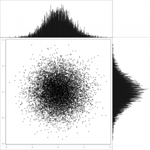
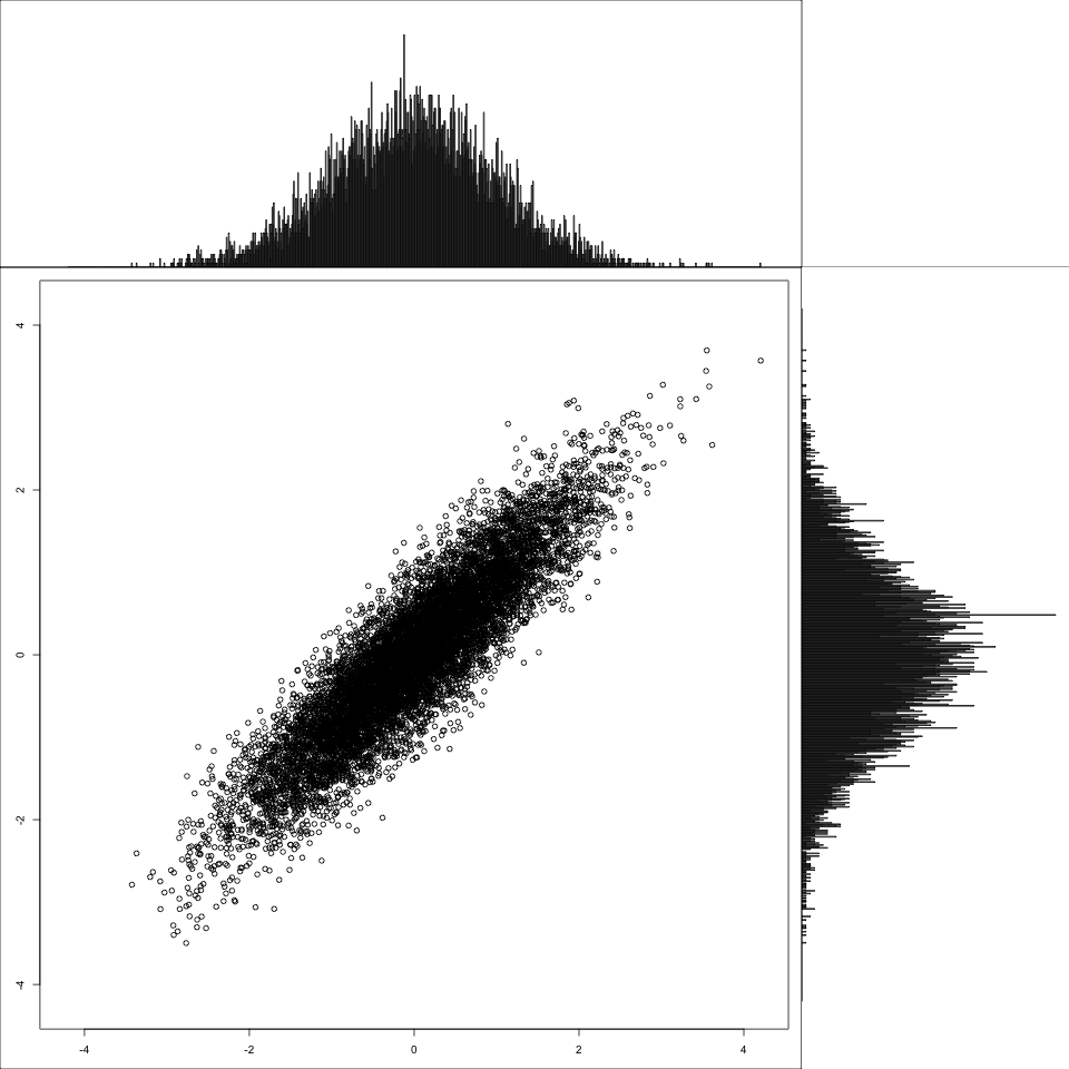
Now, let’s show off what I originally wanted to do: display a plot of two dimensions of a distribution, along with the marginal distributions. I’m wrapping the functionality up into a function so it’s easy to reuse. I use plot to show the sample and barplot to show the distribution as calculated by hist.

1
2
3
4
5
6
7
8
9
10
11
12
13
14
15
16
17
18
19
20
21
22
23
24
25
26
27
28
29
30
31
32
33
# now lets demonstrate with a plot of the multivariate normal and histograms of the marginal distributions
# use package MASS to get the mvrnorm function

plotWithMarginals <- function(x, y){

# find min / max on each dimension
# then set up breaks so that even if x, y are on very different ranges things work
mm <- max(abs(range(x, y)))
breaks <- seq(-mm, mm, by=(2*mm)/1000)

hist0 <- hist(x, breaks=breaks, plot=F)
hist1 <- hist(y, breaks=breaks, plot=F)

# create a grid and check it out to make sure that it's what we want
pp <- layout(matrix(c(2,0,1,3), 2, 2, byrow=T), c(3,1), c(1,3), T)
layout.show(pp)

rang <- c(-mm, mm)

par(mar=c(3,3,1,1))
plot(x, y, xlim=rang, ylim=rang, xlab='', ylab='')

# now plot marginals
top <- max(hist0$counts, hist1$counts)
par(mar=c(0,3,1,1))
barplot(hist0$counts, axes=F, ylim=c(0, top), space=0)

par(mar=c(3,0,1,1))
barplot(hist1$counts, axes=F, xlim=c(0,top), space=0, horiz=T)
}

# mvrnorm <-- sample from a multivariate normal distn
library(MASS)

Now that all the prep is done, this shows a multivariate normal distribution with no correlation between the two variables. Note the shape of the marginal distributions.

1
2
3
eye2 <- matrix(c(1,0,0,1), 2, 2)
sample <- mvrnorm(n=10000, mu=c(0,0), Sigma=eye2)
plotWithMarginals(sample[,1], sample[,2])

plot12.05

And finally, for contrast, a correlated multivariate normal.

1
2
3
yescorr <- matrix(c(1, 0.9, 0.9, 1), 2, 2, byrow=T)
sample <- mvrnorm(n=10000, mu=c(0,0), Sigma=yescorr)
plotWithMarginals(sample[,1], sample[,2])

Querying Databases in R

One of the first things you’ll want to do in R is set it up to talk to databases. The easiest way to do this is using ODBC, via package RODBC.

To get the package, run `

> install.packages(RODBC)

`

Once you have RODBC installed, you call it in R as follows. But it’s very simple: a bit of setup, then sqlQuery will run your sql and return the results in a data frame. `

library(RODBC)

db <- odbcConnect( dsn='your dsn name' )
sql <- 'select page_id, count(*) as cnt
           from document_ads
           group by page_id
           having count(*) > 1'

results <- sqlQuery(db, sql, errors=T, rows_at_time=1024)
str(results)
'data.frame':   282432 obs. of  2 variables:
 $ page_id: int  17646774 17115332 17606022 15899428 17099174 17283774 8604200 16315025 17259751 17283270 ...
 $ cnt            : int  489 1119 132 113 148 200 112 121 1135 633 ...

`

On Windows, you setup the DSNs in the ODBC Data Sources inside the control panel; on MacOS, mysql includes a program called ODBC Administrator; on linux, you’ll have to install unixODBC .

Also, it’s often convenient to write code that caches your query results, particularly if the query takes a while. I’ve found that the easiest thing to do is write the results into a data file and check for the file existence like such: `

filename <- 'query cache.RData'
if (!file.exists(filename)){
   # don't have a cached copy so run the query
   library(RODBC)
   [snip]
   query1 <- sqlQuery(db, sql, errors=T, rows_at_time=1024)

   # save the query results for the future
   save(list=c('query1', 'sql'), file=filename)
   rm(list=c('query1', 'sql') )
}
load(file=filename)

</code

MySQL, Batch Imports, and Rails

I really love Rails, but it’s not the most performant code in the world. Though it doesn’t often arise in CRUD programming, if you do any sort of stats, ML, or data analytics, you’ll frequently find yourself wanting to import lots of data into your db. You could create an ActiveRecord object for each row, but this is glacial, requiring one round trip to the db server per row, and is likely to abuse the kindness of your dba. Instead, there is a wonderful gem called ar-extensions that allows you to access mysql’s native bulk import facilities. To use it you just call Model.import with arrays of data and their corresponding fields. For example, say I have a table like this:

1
2
3
4
5
6
7
8
9
10
11
12
13
14
15
16
17
18
mysql> describe adsense_analytics_days;
+------------------+----------+------+-----+---------+----------------+
| Field            | Type     | Null | Key | Default | Extra          |
+------------------+----------+------+-----+---------+----------------+
| id               | int(11)  | NO   | PRI | NULL    | auto_increment | 
| page_id          | int(11)  | NO   | MUL | NULL    |                | 
| impressions      | int(11)  | YES  |     | NULL    |                | 
| clicked          | int(11)  | YES  |     | NULL    |                | 
| ecpm             | float    | YES  |     | NULL    |                | 
| ctr              | float    | YES  |     | NULL    |                | 
| cpc              | float    | YES  |     | NULL    |                | 
| revenue          | float    | YES  |     | NULL    |                | 
| start_date       | date     | YES  | MUL | NULL    |                | 
| end_date         | date     | YES  |     | NULL    |                | 
| created_at       | datetime | YES  |     | NULL    |                | 
+------------------+----------+------+-----+---------+----------------+
11 rows in set (0.09 sec)
mysql>

This has a corresponding model AdsenseAnalyticsDay. Batch importing with rails is then trivial:

1
2
3
4
5
6
7
8
9
10
11
12
13
14
15
16
17
18
19
20
21
22
23
24
25
require 'ar-extensions'
require 'ar-extensions/import/mysql'

# instead of
if false
  rows.each do |row|
    AdsenseAnalyticsDay.create( ) # etc
  end
end

# you can accomplish a bulk import from, eg, a csv as such:
f = File.new('bulk_import.csv', 'r')
data = []
while line = f.gets
  puts "#{line}" if rand(1000) >= 999
  # pid, impr, clicked, ecpm, ctr, cpc, revenue, start_date, end_date, created_at
  d = line.split(',')
  (0..2).each{ |i| d[i] = d[i].to_i  }
  (3..6).each{ |i| d[i] = d[i].to_f }
  data << d[0..8]
end
f.close

fields = [:page_id, :impressions, :clicked, :ecpm, :ctr, :cpc, :revenue, :start_date, :end_date]
AdsenseAnalyticsDay.import(fields, data, {:validate => false })

where the csv looks like:

1
2
3
4
5
6
7
8
9
10
11
12
$ head bulk_import.csv
0,344,5,0.755814,0.0145349,0.052,0.26,2009-08-06,2009-08-06,2009-08-10 19:49:12
1,8,1,0,0.125,0,0,2009-08-06,2009-08-06,2009-08-10 19:49:12
2,32,9,76.875,0.28125,0.273333,2.46,2009-08-06,2009-08-06,2009-08-10 19:49:12
4,16,1,1.875,0.0625,0.03,0.03,2009-08-06,2009-08-06,2009-08-10 19:49:12
6,17,2,8.82353,0.117647,0.075,0.15,2009-08-06,2009-08-06,2009-08-10 19:49:12
12,15,1,80,0.0666667,1.2,1.2,2009-08-06,2009-08-06,2009-08-10 19:49:12
34,5,0,0,0,0,0,2009-08-06,2009-08-06,2009-08-10 19:49:12
36,2,0,0,0,0,0,2009-08-06,2009-08-06,2009-08-10 19:49:12
39,46,2,11.7391,0.0434783,0.27,0.54,2009-08-06,2009-08-06,2009-08-10 19:49:12
41,3,0,0,0,0,0,2009-08-06,2009-08-06,2009-08-10 19:49:12
$

R Dates - Recovering and Converting From Integers

One problem with R is that dates (class Date) are internally stored as integer numbers of days elapsed since 1 January 1970 and R sometimes loses the dateness of the variables and thinks of it only as an integer. So in the first line, we take the range of dates present in our data, allowing for the fact that some may be skipped. These are just integers — try looking at the output from min(m2$day):max(m2$day). To turn these back into dates we add them to the first date object: `

> min(m2$day):max(m2$day)
 [1] 14245 14246 14247 14248 14249 14250 14251 14252 14253 14254 14255 14256 14257 14258 14259 14260 14261 14262 14263 14264 14265 14266 14267 14268 14269 14270 14271
[28] 14272 14273 14274 14275 14276 14277 14278 14279 14280 14281 14282 14283 14284 14285 14286 14287 14288 14289 14290 14291 14292 14293 14294 14295 14296 14297 14298
[55] 14299 14300 14301 14302 14303
>
> as.integer(as.Date('1970-01-01'))
[1] 0
>
> # the fix:
> as.Date('1970-01-01') + min(m2$day):max(m2$day)
 [1] "2009-01-01" "2009-01-02" "2009-01-03" "2009-01-04" "2009-01-05" "2009-01-06" "2009-01-07" "2009-01-08" "2009-01-09" "2009-01-10" "2009-01-11" "2009-01-12"
[13] "2009-01-13" "2009-01-14" "2009-01-15" "2009-01-16" "2009-01-17" "2009-01-18" "2009-01-19" "2009-01-20" "2009-01-21" "2009-01-22" "2009-01-23" "2009-01-24"
[25] "2009-01-25" "2009-01-26" "2009-01-27" "2009-01-28" "2009-01-29" "2009-01-30" "2009-01-31" "2009-02-01" "2009-02-02" "2009-02-03" "2009-02-04" "2009-02-05"
[37] "2009-02-06" "2009-02-07" "2009-02-08" "2009-02-09" "2009-02-10" "2009-02-11" "2009-02-12" "2009-02-13" "2009-02-14" "2009-02-15" "2009-02-16" "2009-02-17"
[49] "2009-02-18" "2009-02-19" "2009-02-20" "2009-02-21" "2009-02-22" "2009-02-23" "2009-02-24" "2009-02-25" "2009-02-26" "2009-02-27" "2009-02-28"
>

`

Shading Pieces of an R Plot

This is post #11 in a running series about plotting in R.

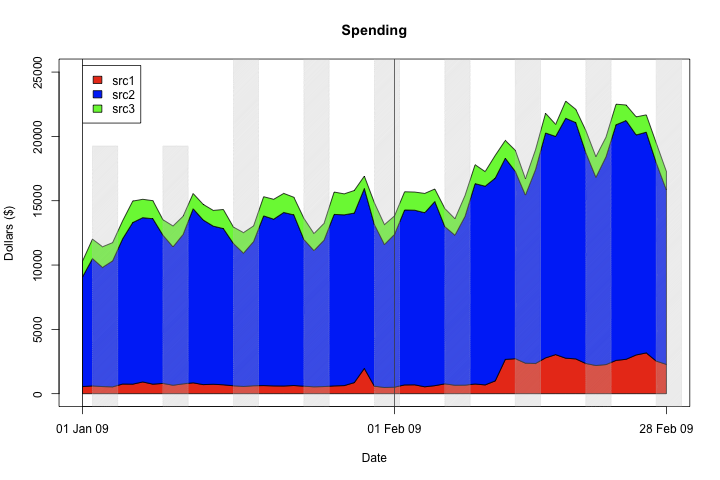
I often want to shade pieces of an R plot, in order to visually draw out some piece, such as weekends or recessions. Let’s look at how to do that with the plain plotting tools.

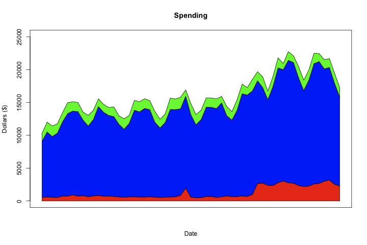
First, I have some obscured data from work. I’m going to take 3 series and turn them into stacked filled line plots. But first, let me show you where we’re going to end up:

First, let’s grab some data: post11.data and prep it, which basically involves making R understand that the day column is a date.

1
2
m2 <- read.csv(file='post11.data.csv', header=T, sep=',')
m2$day <- as.Date(as.character(m2$day))

Now that that’s over, let’s just plot the 3 stacked series. The basic technique, as mentioned in the last post, is constructing polygons with our desired boundaries.

1
2
3
4
5
6
7
8
9
10
11
12
ylim <- c(0, 1.1*max(m2$src1 + m2$src2 +  m2$src3))
xx <- c(m2$day, rev(m2$day))
yysrc2 <- c(rep(0, nrow(m2)), rev(m2$src2))
plot(x=m2$day, y=m2$src2, ylim=ylim, col='red', type='l', xaxt='n',
ylab='Dollars ($)', xlab='Date', main='Spending')
polygon(xx, yysrc2, col='red')

yysrc1 <- c(m2$src2, rev(m2$src2) + rev(m2$src1))
polygon(xx, yysrc1, col='blue')

yysrc3 <- c(m2$src2 + m2$src1, rev(m2$src2) + rev(m2$src1) + rev(m2$src3))
polygon(xx, yysrc3, col='green')

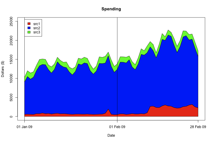
And let’s add some prettying up: a legend and X axis labels on the first of the month and the last data point present. Note that this code is generic, so it will work on arbitrary date ranges, including spanning years, date ranges that don’t end on the last day of a month, etc.

1
2
3
4
5
6
7
8
9
10
11
12
13
14
# x axis labels
labdates <- as.Date('1970-01-01') + min(m2$day):max(m2$day)
labdates <- labdates[ format(labdates, '%d') == '01']
labdates <- unique(c(labdates, max(m2$day)))

labnames <- format(labdates, '%d %b %y')
axis(1, at=labdates, labels=labnames)

# black lines first day of month
for(a in labdates[ format(labdates, '%d') == '01']){
abline(v=a)
}

legend(x=m[1,]$day, y=ylim[2]+500, c('src1', 'src2', 'src3'), fill=c('red', 'blue', 'green'))

Now, let’s shade the background. What I’m going to do is draw semi transparent grey boxes over Saturday and Sunday. There are a couple issues to be careful of: first, we don’t want to do this over the legend, so we make the first couple of rectangles shorter. Second, we find weekends by looking for Saturday, but the first day of data present could start on Sunday, so we have to check that as well. The rect command draws the specified distance left and right (where -1 equals minus one day, since the data is formatted as Date), as well as top and bottom.

1
2
3
4
5
6
7
8
9
10
11
12
13
14
15
16
17
18
19
20
# make the first 3 lower to avoid our legend
cnt <- 0

# set alpha = 80 so it's relatively transparent
color <- rgb(190, 190, 190, alpha=80, maxColorValue=255)

# check if the first data point is a Sunday
m2$dow <- format( m2$day, '%a' )
lhs <- m2[1,'dow']
if(lhs == 'Sun'){
a <- m2[1,]$day
rect(xleft=a-1, xright=a+2 - 1, ybottom=-1000, ytop=1.1*ylim[2] * ifelse(cnt < 2, 0.7, 1), density=100, col=color)
cnt <- cnt + 1
}

# plot 2-day width rectangles on every Saturday
for( a in m2[ m2$dow == 'Sat', ]$day ){
rect(xleft=a-1, xright=a+2 - 0.5, ybottom=-1000, ytop=1.1*ylim[2] * ifelse(cnt < 2, 0.7, 1), density=100, col=color)
cnt <- cnt + 1
}

Finally, I added a quick set of dashed (lty=3) horizontal rules. This makes it much easier to read on projectors. For results, see the first image in this post.

1
2
3
4
5
# dashed grid
horguides <- c(5,10,15,20)* 1000
for(h in horguides){
abline(h=h, col='gray60', lwd=0.5, lty=3)
}

Matt Riley Rides the Zip Line at Scribd

We are trying to speed the zip line up so we attached what is basically a 300 foot rubber band — a tan, 4mm, Thera Band Roll to two columns and shot Matt down the zip line. He flew! Unfortunately, the latex band wasn’t as robust as we would have liked.

Here’s the video of us shooting stuff beforehand: